
Not an investment advice – ACADEMIC PURPOSE ONLY
Why trade trend following, and why on crypto and RWA
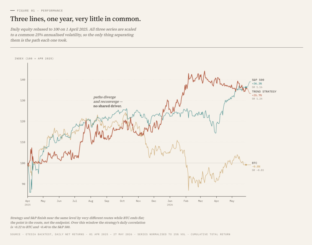
Over the simulated year from April 2025 to April 2026, our trend-following strategy returned 35.3% net with a 1.26 Sharpe ratio, while exhibiting a correlation of -0.22 to Bitcoin and -0.40 to the S&P 500. At equivalent volatility over the same window, BTC buy-and-hold produced a Sharpe of -0.03 and the S&P 500 produced 1.16.
The interesting number is not the return. It is the correlation.
This is the first article in a series introducing Etesia and the strategies we run. We start with trend following because it is the first strategy we have launched and the easiest to explain. Later articles will unpack Sharpe ratio, volatility targeting, and the other pillars of the platform.
What is trend following?
Trend following is a systematic strategy that takes long positions in markets that have been rising and short positions in markets that have been falling. The signal is mechanical, derived from past prices alone, and the rules are the same across every instrument the strategy trades.
A trend follower has no opinion on whether Bitcoin is overvalued, or whether gold should rise on inflation fears. It looks at price history, measures the strength and direction of recent moves, sizes a position to a target risk, and waits. When the trend reverses, the position flips. There is no narrative, no forecast, no view.
This style is often called CTA, for Commodity Trading Advisor, the regulatory label given to firms that have run this approach in futures markets since the 1970s. Names like AHL, Winton, Aspect, Man and Campbell have managed tens of billions in CTA capital for decades. We apply the same framework to a different universe: crypto perpetual swaps and tokenised real-world assets.
How the signal works
The raw material is price, and the question is simple: is this market moving, and in which direction?
The standard way to answer it is to compare two moving averages of the price, one fast and one slow. The fast average tracks recent price closely; the slow average lags. The gap between them is a single number that moves around zero:
– Fast above slow: recent prices sit above older prices. The signal is positive, the market is trending up.
– Fast below slow: the signal is negative, the market is trending down.
– The distance from zero measures trend strength. Near zero means no trend, just noise.
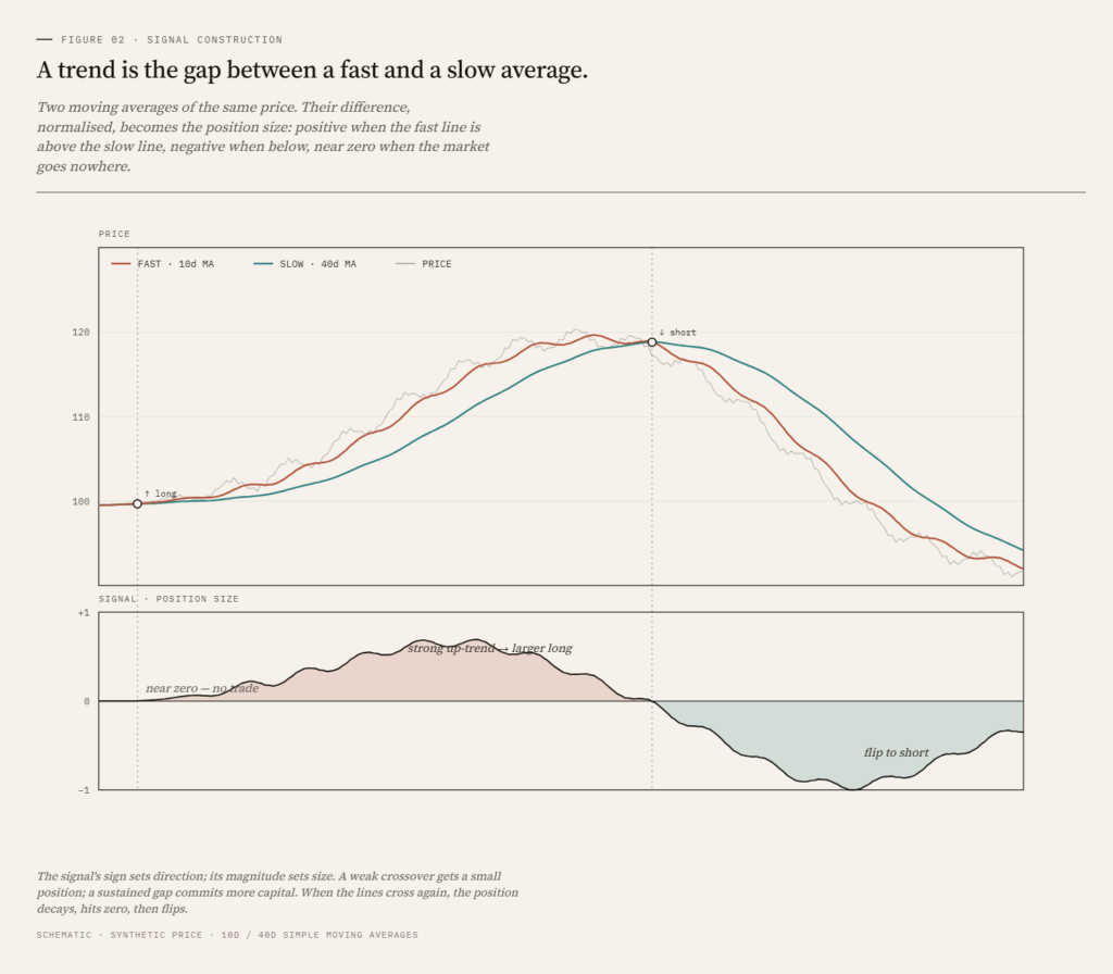
The magnitude does more than give direction; it sets the size of the position. A young, weak trend gets a small position. As the trend persists and the signal grows, the position is scaled up. The strategy commits the most capital to the trends that have proven themselves, and return accumulates for as long as the move lasts. It never has to call the top or the bottom; it needs the move, once underway, to outlast the noise.
When the trend turns, the signal decays toward zero and the position is trimmed. When it crosses zero, the position flips, long to short or short to long. This is the built-in risk control: the signal is its own stop-loss. A position that stops working is cut automatically, and reversed if the move continues against it. Losers are closed by construction; winners are held for as long as the trend runs.
In practice we combine several signals at different speeds, so the strategy responds both to fast multi-day moves and slow multi-month ones. The principle does not change.
How it captures alpha
The result is a characteristic payoff. Most trades are small losses: a signal forms, the trend fails to materialise, the position closes near where it opened. A minority are large gains: a market that trends for weeks or months, with the position scaled up and held the whole way. The few large wins more than cover the many small losses.
This is how trend following captures alpha. Not by forecasting, but by harvesting the moves that persist while bleeding small amounts on those that do not. Why persistent moves exist at all is the subject of the next section.
Takeaway: trend following reads direction and strength from price, scales into trends that prove themselves, and flips when they reverse. The signal is its own stop-loss, which gives the strategy its many-small-losses, few-large-wins payoff.
Why it works
The honest answer is that nobody fully knows. The useful answer is that several reinforcing effects, each modest on its own, combine into a persistent edge.
Slow information diffusion. News and changes in fundamentals do not instantly translate into prices. Different investors update their views at different speeds. As information spreads from informed traders to less informed ones, prices drift in the direction of the new information, producing autocorrelation in returns at multi-week to multi-month horizons.
**Herding and momentum chasing. Investors react to other investors. A move that starts on fundamentals attracts trend chasers, who push the move further, attracting more chasers. This produces overshooting and eventual reversal, but the overshooting phase is exactly what trend following captures.
Risk transfer. Some market participants must trade for reasons other than expected return: hedgers, rebalancers, forced sellers in stress. Their flows are predictable in direction and create persistent pressure that systematic strategies can take the other side of.
Behavioural anchoring. Investors anchor on recent prices, then update slowly. This delays the price response to genuinely new information and stretches moves over time.
There is a fifty-year academic literature on time-series momentum that documents the effect across more than a hundred markets and back to the 19th century. Moskowitz, Ooi and Pedersen (2012) is the standard reference. The effect is not a quirk of one decade or one asset class.
Why this should work especially well in crypto and RWA perpetuals
Crypto markets are younger, more retail-driven, and less crowded with systematic capital than developed equity or rates markets. Narratives drive sustained flows: an ETF approval, a chain upgrade, a regulatory shift, a meme cycle. Information diffuses slowly because the participant base is fragmented across geographies, time zones and platforms. Forced flows from leverage liquidations and scheduled token unlocks are large relative to genuine investment flows. Each of the mechanisms above is more pronounced in crypto than in mature asset classes.
Tokenised RWA add a second layer. Perpetual swaps on metals, energy and equity indices trade 24/7 and respond to global flows, but the underlying assets are driven by macro factors that are independent of crypto. The same trend-following rules, applied to a gold perpetual and to an ETH perpetual, produce signals that move independently of each other.
Takeaway: the economic case for trend following is well documented across decades and asset classes. The case is structurally stronger in crypto and tokenised RWA than in developed markets.
Why it diversifies
This is the part that matters most for anyone already holding crypto, equities or gold.
A trend-following strategy has, by construction, no permanent long bias. It will be long in rising markets and short in falling ones. Over time, its returns depend on whether trends exist, not on whether markets go up. That makes it structurally different from buy-and-hold.
In a stress event, this matters. The 2008 crisis, the 2018 crypto winter, the March 2020 crash, the 2022 bear market: in each, buy-and-hold equity and buy-and-hold crypto fell together. Trend-following CTAs, in aggregate, were flat to positive across most of these episodes, because by the time the crash matured they had flipped short on the assets that were falling.
In our backtest, the realised correlations are -0.22 to BTC and -0.40 to the S&P 500. That is not a coincidence and it is not engineered through optimisation. It is a property of any strategy that responds symmetrically to up and down moves, applied to a universe where directional persistence exists.
For an investor whose portfolio is concentrated in BTC, ETH, equities, gold, or some mix of these, adding an uncorrelated strategy with a similar Sharpe materially improves portfolio efficiency.
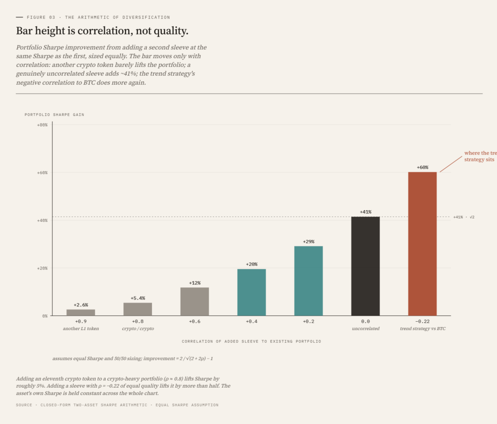
This matters most for crypto natives, for a reason that is easy to miss. A portfolio holding BTC, ETH, an L1 or two and a basket of tokens feels diversified. It is not. Daily return correlations across major crypto assets, held outright, routinely sit between 0.7 and 0.9: when BTC sells off, the rest sell off with it. Ten correlated tokens behave, in risk terms, close to a single position, and the eleventh adds almost nothing. However many names it holds, a crypto-native portfolio is usually one bet.
The arithmetic of diversification makes the point precise. Combine two assets of equal Sharpe and zero correlation, split evenly, and portfolio Sharpe rises by a factor of √2, a gain of 41%, because the volatilities partly offset while the returns still add. Correlation is what governs that gain. Run the same calculation on two assets correlated at 0.8, the crypto-to-crypto case, and the improvement collapses to about 5%. The correlation absorbs almost everything diversification would otherwise give you. This is why buying another token does so little.
The trend-following strategy sits at the other end of that scale. Its backtested correlation to BTC is -0.22, below zero rather than near it, so the same arithmetic gives more than √2: close to 1.75x at equal Sharpe, and a reduction in drawdown rather than a dilution of return. For an investor who is 70% or more in crypto, this is the position that changes the portfolio. The first genuinely uncorrelated sleeve is worth more than every correlated token added after it.
Takeaway: the diversification benefit comes from a different return profile, not another asset. Holding more crypto does not replicate it, however many tokens it is spread across.
How Etesia runs the strategy
The strategy operates on a universe of perpetual swaps across ten sectors: DeFi, Layer-1, Infrastructure, Meme, Payment, Store of Value, AI, Energy, Equity Indices and Metals. Three of those sectors (Energy, Equity Indices, Metals) are tokenised real-world assets. The remainder are crypto-native. Cross-sector daily return correlations are frequently below 0.2.
The processing pipeline follows standard institutional CTA conventions, adapted for the crypto execution environment
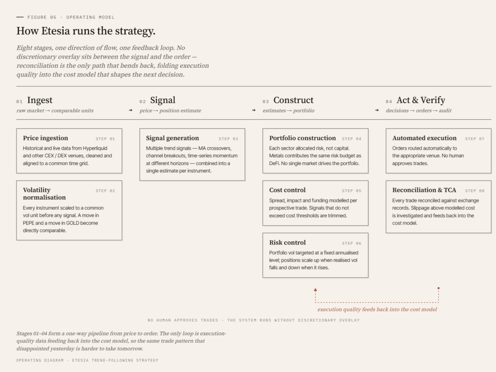
The full system runs without discretionary overlay. We do not override the signal because we have a view on the macro environment. The point of a systematic strategy is to harvest a statistical edge consistently across thousands of trades, not to be right about any one of them.
Takeaway: the strategy follows institutional CTA conventions. The novelty is the universe (crypto plus tokenised RWA on perpetuals) and the execution stack (on-chain native), not the signal logic.
What the strategy delivered in backtest
For the period from April 2025 to April 2026, simulated on Hyperliquid execution data with realistic cost assumptions
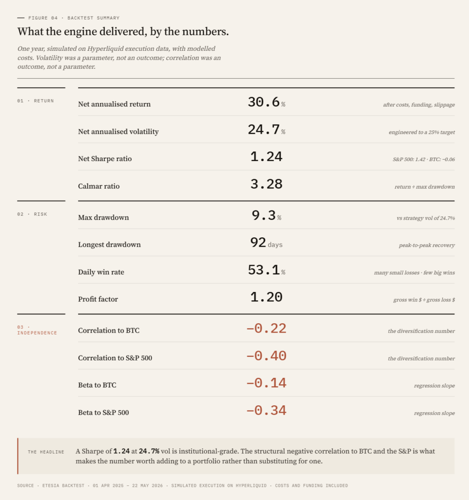
Sector contribution was concentrated in three areas: Metals (37% of PnL), Layer-1 (25%) and DeFi (17%). The remaining seven sectors contributed the balance. Highest sector Sharpe ratios were Metals (1.10), Layer-1 (0.90) and DeFi (0.76).
The Sharpe ratio of 1.11 is the headline number for anyone who follows quantitative finance. What it means in plain terms, and how it compares to strategies most readers already know, is the subject of the next article in this series. Briefly: a Sharpe above 1 is considered good. Most discretionary hedge funds operate in the 0.3 to 0.7 range over multi-year periods. Over the same backtest window, BTC buy-and-hold produced a Sharpe of -0.03 and the S&P 500 produced 1.16.
The 25% volatility is a parameter we choose, not an output. The strategy is built to deliver a fixed annualised volatility. We have set it at 20% to match the risk profile most crypto holders are already comfortable with. The same engine can run at 10% or 40%, with returns scaling roughly linearly. This trade-off between target volatility and expected return is the subject of the third article in the series.
Takeaway: at our chosen risk budget, the backtest returned 30.6% with a 1.26 Sharpe and structural negative correlation to both crypto and equity benchmarks.
Previous performances do not predict future performances
This is a backtest. Backtests are not live performance. Costs are modelled with care, but live execution will reveal frictions that simulation cannot capture. We expect the live Sharpe to be lower than the simulated Sharpe. Anyone who tells you otherwise has not run live systematic strategies before.
Trend following has bad years. The 2010s decade was difficult for most CTAs, with range-bound rates and commodity markets that produced few sustained trends. A strategy that targets fixed volatility will, by construction, take losses comparable to its volatility in any year that trends are absent. A 20% volatility strategy can lose 10% to 20% in a poor year without anything being wrong with the model.
Our edge is not a signal nobody else has found. The edge sits in three places: a universe that few systematic teams trade today (RWA perpetuals next to crypto), an execution stack that runs natively on-chain, and the application of institutional risk discipline to a market where most participants run leveraged directional bets without it.
Takeaway: expect a Sharpe near 1 over multi-year horizons, with single-year outcomes that can range widely. The strategy is designed to be held alongside other exposures, not as a standalone bet.
Who this is for, and how to access it
The strategy fits two profiles:
– Holders of directional exposure (crypto, equity, gold) who want to reduce portfolio concentration without exiting their core positions.
– Allocators with a dedicated alternatives bucket who want crypto-native systematic exposure delivered through institutional infrastructure.
Access is through three channels:
– Tokenised vault on Hyperliquid. Deposit and withdraw on-chain. ERC-4626/7540 compatible vaults are live and in pre-release.
– Separately managed accounts. For larger allocators with custom mandates or reporting requirements.
– Institutional platforms. Distribution partnerships are in progress.
Etesia is non-custodial by design. Investor assets remain in on-chain vault structures at all times. No client capital flows through the corporate entity.
*The next article in this series unpacks Sharpe ratio: what it measures, how to read it, and why a strategy with a Sharpe of 1 can still have a bad year. The one after that explains volatility targeting, and what it means to choose a risk level rather than try to forecast returns.*
*Past performance and backtested results are not indicative of future results. Backtest results are based on simulated execution on Hyperliquid and include estimated trading costs and fees. Actual performance may differ materially. This article does not constitute an offer or solicitation to invest.*